
meta-vlm
About
Add a short description of your repository
Wiki
Overview
This repository provides surrogate aerodynamic models for unswept and untwisted wings, developed from Vortex Lattice Method (VLM) simulations.
The models are intended to provide a fast, compact representation of spanwise aerodynamic characteristics for use in preliminary aircraft design, parametric studies, optimization, and other applications where repeated aerodynamic evaluations are required.
Instead of running a VLM analysis for every combination of wing geometry and angle of attack, the models allow the relevant aerodynamic quantities to be reconstructed from a small set of metamodels based primarily on the wing aspect ratio (AR), taper ratio (TR), and spanwise coordinate η.
The repository provides a set of relations that can be directly reused to evaluate these models and reconstruct the corresponding aerodynamic coefficients.
Scope and Assumptions
The models in this repository are applicable to unswept, untwisted finite wings analyzed using the Vortex Lattice Method (VLM). The current model set is based on the following assumptions:
- Wing geometry: unswept and untwisted wing with a prescribed taper ratio and aspect ratio.
- Airfoil: models are provided for several airfoil geometries. The alpha-independent parameters , , and kα can be used from the symmetric-airfoil response, while camber effects are captured by additional parameters described in the Methodology section.
- Computation method: the reference data are generated using VLM (from Aerosandbox library) and therefore inherit its assumptions, including inviscid, incompressible, potential-flow aerodynamics and the absence of viscous/profile-drag effects.
- Spanwise coordinate: aerodynamic quantities are represented as functions of the normalized spanwise coordinate η.
- Angle of attack: the aerodynamic dependence on alpha is represented by analytical relations obtained by post-processing the VLM results.
- Parameter domain: AR, TR, and η should remain within the ranges covered by the corresponding SplineCloud models.
- Flow regime: the models describe the linear/potential-flow regime represented by the underlying VLM solutions and should not be used to predict stall or other strongly nonlinear viscous phenomena without coupling with viscous 2D solutions.
Methodology
The methodology is aimed at building a reusable library of surrogate models capable of predicting VLM aerodynamic results for families of wing geometries and different airfoils. The resulting models are intended to provide a fast source of aerodynamic data that can be coupled with other aerodynamic models, including 2D viscous airfoil solutions, to estimate the spanwise distribution of aerodynamic coefficients with substantially lower computational cost than high-fidelity methods such as RANS.
The methodology consists of three main stages:
- Generation and processing of a systematic VLM dataset;
- Discovery of analytical relations that describe the dependence of aerodynamic coefficients as functions of eta on angle of attack;
- Construction of the reusable response surfaces for alpha-normalized parameters on SplineCloud;
- Construction of 3-parameter meta-models m(AR, TR, eta) from 2D response surfaces (either by volumetric lofting or interpolation).
The resulting 3-parameter meta-models in combination with analytical angle-of-attack dependencies are used for prediction of the VLM outputs with high accuracy (with average relative error below 5%).
VLM Analysis
This repository contains datasets of VLM solutions, generated for a family of finite-wing geometries. The principal geometric parameters considered are:
- aspect ratio, AR;
- taper ratio, TR;
- spanwise coordinate, η;
- airfoil geometry (camber);
- angle of attack, α.
For each combination of these parameters, the VLM solver provides the circulation distribution and aerodynamic forces from which the required sectional aerodynamic quantities are calculated.
The circulation-based sectional lift coefficient is defined as:
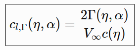
where Г is the local circulation, V_inf is the freestream velocity, and c(η) is the local chord.
The aerodynamic sectional lift and induced-drag coefficients, and are obtained from the forces calculated by the VLM solution. The circulation-based and force-based coefficients are retained as separate quantities because they describe different stages of the VLM solution and exhibit slightly different dependencies on angle of attack. The repository with VLM datasets therefore initially represents the aerodynamic response as a multidimensional relation of the general form

The subsequent analysis identifies which parts of this dependence can be represented analytically and which require fitting spline models.
Alpha Reduction
A key observation from the VLM data is that a substantial part of the variation with angle of attack can be represented by simple analytical functions. The purpose of alpha reduction is therefore to analytically exclude the influence of the angle of attack, and model planform parameters influence on aerodynamic coefficients distribution over the wing span.
Circulation-based lift coefficient
For symmetric airfoils, the circulation-based sectional lift coefficient exhibits an almost exact dependence on sin(alpha).
The corresponding normalized quantity is defined as
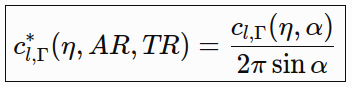
where the factor 2pi provides normalization relative to the classical thin-airfoil lift slope. The important result is that is independent of alpha (with very high accuracy), allowing it to be represented by a lower-dimensional alpha-independent meta-model.
Aerodynamic lift coefficient
The lift coefficient calculated from the aerodynamic forces exhibits a related but slightly different nonlinear dependence on angle of attack. The observed behavior can be represented using the correction
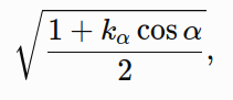
where kα is a geometry-dependent parameter.
The normalized aerodynamic lift coefficient is therefore defined as:
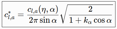
The parameter kα is modeled as:
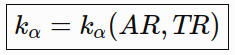
and is therefore independent of η and α within the current model formulation.
Induced drag coefficient
The VLM results show that the sectional induced-drag coefficient follows an approximately universal angular dependence of sin2(α)*cos(α).
Thus, its normalized quantity can be expressed as
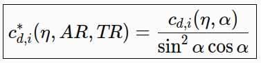
which is approximately independent of α.
This relation is consistent with the familiar quadratic behavior of induced drag at small angles of attack while retaining the additional nonlinear angular dependence observed in the VLM results.
Airfoil and Camber Effects
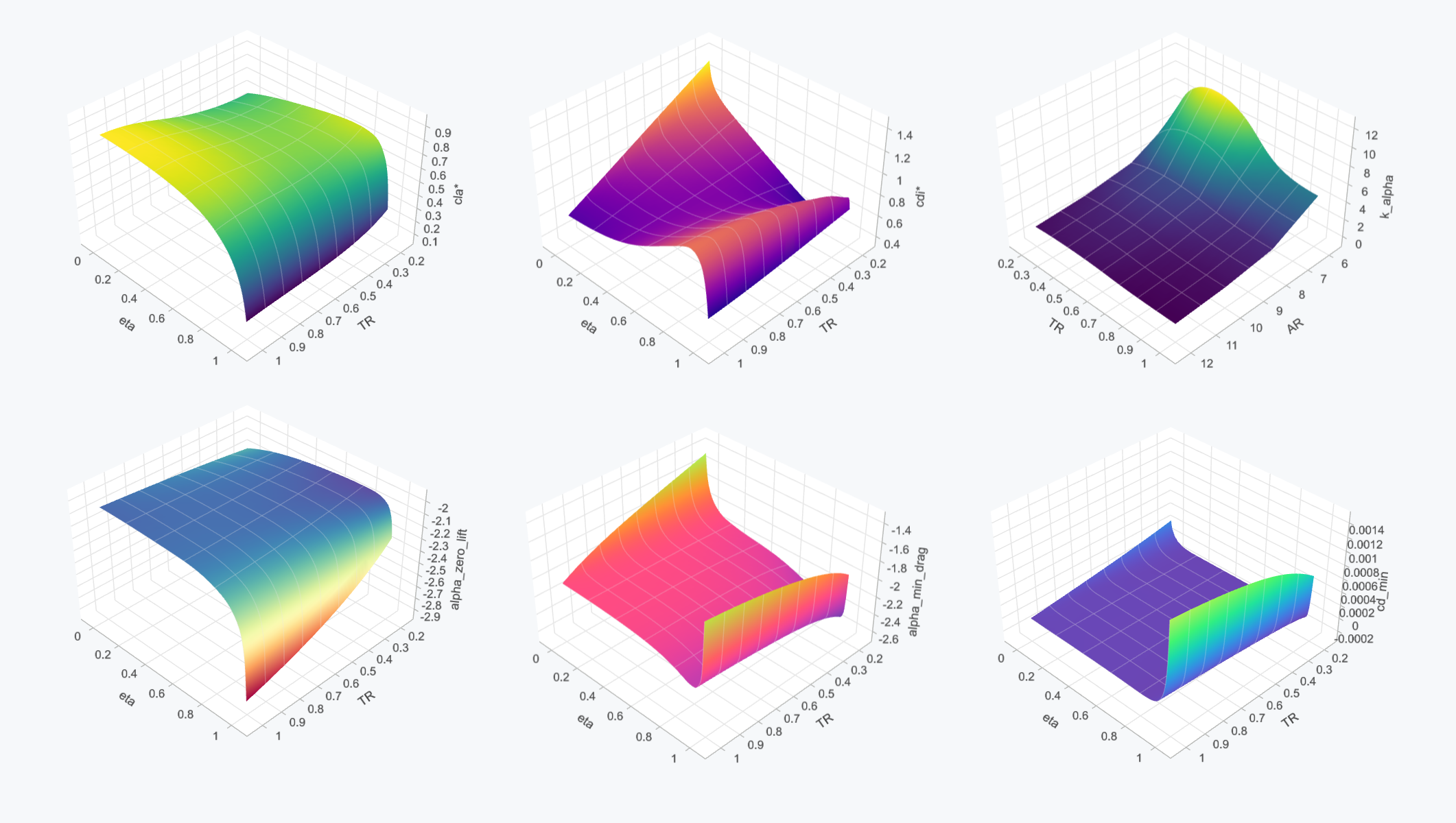
The analysis of several airfoils showed that the main alpha-independent aerodynamic parameters can be separated from airfoil-specific effects. In particular, the symmetric-airfoil response provides a useful baseline for the quantities: , , , kα.
Effects associated with airfoil camber are represented through additional parameters that modify the baseline response.
Zero-lift angle
For a cambered airfoil, the local aerodynamic response is shifted along the angle-of-attack axis. This shift is represented by the local zero-lift angle
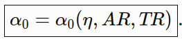
The zero-lift angle therefore becomes one of the quantities included in the meta-model library for cambered airfoils.
Minimum-drag condition
The induced-drag response of a cambered airfoil can exhibit a shifted minimum. This is represented by

and non-zero minimal induced drag coefficient

These quantities allow the cambered-airfoil response to be reconstructed from the symmetric-airfoil baseline while accounting for the observed spanwise variation of the drag minimum.
The detailed analytical reconstruction of the cambered-airfoil coefficients is described in Section 4.3.
Normalized Aerodynamic Quantities
After extracting the dominant angle-of-attack dependence, the following quantities are retained as alpha-independent model parameters:
- - Normalized aerodynamic lift coefficient
- - Normalized induced-drag coefficient
- - Normalized circulation-based lift coefficient
- kα - Correction parameter for nonlinear lift dependence on alpha
- α0 - Local zero-lift angle
- αmin drag - Local angle of minimum induced drag
- - Minimum induced-drag coefficient
The first four quantities describe the principal alpha-independent aerodynamic response, while α0, αmin drag, and provide the additional corrections required to reconstruct the response for different airfoils.
Construction of Response Surfaces
For each normalized parameter, VLM results are processed at multiple combinations of AR, TR, and eta. Once the alpha dependence has been removed, each parameter becomes a three-dimensional relation of the form
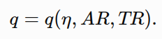
Models are represented as a collection of 2D spline surfaces that by lofting (or interpolation) can be converted into 3-parameter models using built-in methods of the SplineCloud client library.
For a fixed value of AR, for example,
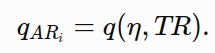
These surfaces form the basic reusable elements stored in this repository.
An important property observed in the VLM data is that the modeled quantities generally exhibit lower nonlinearity in the AR direction than in the TR direction. Therefore, TR is retained as one of the surface coordinates, while the surfaces are lofted along AR. This choice provides greater control over spline complexity and helps reduce the risk of overfitting while retaining the nonlinear dependence on taper ratio.
Volumetric Lofting
The collection of 2D response surfaces can be combined into a three-dimensional relation using the volumetric lofting functionality of the SplineCloud client library.
The resulting object is a trivariate spline metamodel that can be evaluated at arbitrary combinations of η, TR, and AR within the model domain.
The complete methodology can therefore be summarized as:
VLM analysis -> airfoil-specific datasets -> normalized parameters -> collection of spline surfaces per aspect ratios -> 3-parameter meta-models
The resulting metamodel library provides the geometry- and airfoil-dependent parameters required to reconstruct the aerodynamic response without repeatedly running the underlying VLM analysis
Meta-Model Reuse
The aerodynamic models are provided as SplineCloud surfaces, accessible by their unique IDs. These surfaces can be accessed and reconstructed in Python code using the splinecloud-scipy client library.
For each modeled parameter, a set of 2D response surfaces is provided for several discrete aspect-ratio values,

Each surface represents a relation between the spanwise coordinate and taper ratio,
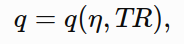
at a particular AR. Surface IDs for each parameter and the corresponding AR values are provided in Section 4.1.
The collection of surfaces can be combined in code to construct a trivariate metamodels
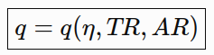
by lofting or interpolating between the available AR surfaces using built-in methods of the splinecloud-scipy library. This allows the resulting model to be evaluated at arbitrary eta, TR and AR combinations. Extrapolation is supported but can not be trusted in far regions.
Two implementations are available in splinecloud-scipy library:
- LoftedSplineVolume — constructs a continuous spline volume from the supplied surfaces;
- InterpolatedSplineVolume — interpolates between the supplied surfaces.
The , , and kα surfaces generated from the symmetric airfoil can also be used to predict aerodynamic coefficients for cambered airfoils. The analysis of the investigated airfoils showed that the relative difference between these normalized parameters is below 1%, indicating that their dependence on wing geometry and spanwise position is effectively independent of airfoil camber within the investigated cases. The effects of camber are therefore captured separately through the camber-produced parameters α0, αmin drag , and .
Response Surface Collections
Symmetric Airfoil (NACA 0009)
cla_norm:
  AR=6:  "srf_8E0ui4ABe5st"
  AR=8:  "srf_IA936WqOzbyy"
  AR=10: "srf_8ee5vCk1WlMM"
  AR=12: "srf_cPn2USXrFGJ8"

cdi_norm:
  AR=6:  "srf_XpVmfL6KnJ6w"
  AR=8:  "srf_3RHqnbRA4CVE"
  AR=10: "srf_kAFftyq2wzXh"
  AR=12: "srf_k4qFTbVbeY0X"

k_alpha: "srf_HlJGtB8WtDpM"
Cambered Airfoil (NACA 2412)
alpha_zero_lift:
  AR=6:  "srf_NBNdYKZn8GtU"
  AR=8:  "srf_QA10Lzf50Ui8"
  AR=10: "srf_xLIvj9wdyue1"
  AR=12: "srf_drsjDl6Fej7p"

alpha_min_drag:
  AR=6:  "srf_9Kks85S88upO"
  AR=8:  "srf_KNmPne6tXIV3"
  AR=10: "srf_PKjODc1nBCqo"
  AR=12: "srf_eWAdznD8hI7G"

cdi_min:
  AR=6:  "srf_4HHZ7LWfoFHL"
  AR=8:  "srf_q2258c4RHiBC"
  AR=10: "srf_Gan1gGndY5iX"
  AR=12: "srf_NQVYZi7o3IZG"
Prediction of Aerodynamic Coefficients
The trivariate metamodels provide the alpha-independent aerodynamic parameters as functions of wing geometry and spanwise position. For a given wing geometry and angle of attack, these parameters are combined with the corresponding analytical angle-of-attack relations to reconstruct the sectional aerodynamic coefficients.
Symmetric airfoil
For a symmetric airfoil, the aerodynamic coefficients are reconstructed using the following relations.
The circulation-based lift coefficient is

and the aerodynamic lift coefficient is

The induced-drag coefficient is

Thus, for a symmetric airfoil, the angle-of-attack dependence is introduced analytically, while the remaining quantities are obtained directly from the trivariate metamodels.
Cambered airfoil
For a cambered airfoil, the symmetric-airfoil baseline parameters , , and kα can be reused. The effect of camber is introduced through the additional metamodels α0, αmin drag, .
The lift coefficient relations are shifted by the local zero-lift angle,

The aerodynamic lift is therefore reconstructed as

while the corresponding circulation-based lift is

For induced drag, the cambered-airfoil response is represented relative to its local minimum-drag angle. Define

The reconstructed induced-drag coefficient is

Here, all quantities on the right-hand side are evaluated at the requested eta, TR, AR.
This formulation separates the aerodynamic response into two components: planform-dependent and camber-dependent.
Practical evaluation sequence
For a requested point (eta, AR, TR, alpha):
1. Evaluate the required trivariate meta-models at (eta, TR, AR).
2. Evaluate kα(AR,TR).
3a. For a symmetric airfoil, apply the corresponding analytical alpha-relations directly.
3b. For a cambered airfoil, evaluate α0, αmin drag, and , then apply the shifted analytical relations.
The resulting aerodynamic coefficients evaluated for a range of eta values provide the predicted spanwise aerodynamic distribution without requiring a new VLM solution.
Examples
Constructing a lofted meta-model
The following example uses the normalized aerodynamic lift coefficient.
from splinecloud_scipy import LoftedSplineVolume

cla_norm_surfaces = {
    "AR=6":  "srf_XXXXXXXXXXXX",
    "AR=8":  "srf_XXXXXXXXXXXX",
    "AR=10": "srf_XXXXXXXXXXXX",
    "AR=12": "srf_XXXXXXXXXXXX",
}

AR_values = [int(key.split("=")[1]) for key in cla_norm_surfaces]

surf_uids = list(cla_norm_surfaces.values())

cla_norm_model = LoftedSplineVolume(surf_uids, AR_values)
The resulting model can be evaluated as
cla_norm = cla_norm_model.eval(eta, TR, AR)
For example:
cla_norm = cla_norm_model.eval(0.3, 0.5, 11)
Using an interpolated volume
Alternatively, the surfaces can be combined using InterpolatedSplineVolume:
from splinecloud_scipy import InterpolatedSplineVolume

cla_norm_model = InterpolatedSplineVolume(surf_uids, AR_values)

cla_norm = cla_norm_model.eval(0.3, 0.5, 11)
Reconstructing aerodynamic coefficients
Once the required normalized parameters have been evaluated, the original aerodynamic coefficients can be reconstructed using the analytical alpha relations.
For example, for symmetric airfoil:
from numpy import pi, sin, cos, sqrt
alpha = np.radians(5.0)

cla_norm = cla_norm_model.eval(eta, TR, AR)

cl_aero = 2*pi  * cla_norm * sin(alpha) * sqrt((1 + k_alpha * cos(alpha)) / 2)

cdi_norm = cdi_norm_model.eval(eta, TR, AR)

cdi = cdi_norm * sin(alpha)**2  * cos(alpha)
For a cambered airfoil, the additional metamodels are evaluated first to obtain the local zero-lift angle, minimum-drag angle, and minimum induced-drag coefficient:
alpha = np.radians(5.0)

# Zero-lift angle
alpha_zero_lift = alpha_zero_lift_model.eval(eta, TR, AR)

# Minimum-drag angle
alpha_min_drag = alpha_min_drag_model.eval(eta, TR, AR)

# Minimum induced drag
cdi_min = cdi_min_model.eval(eta, TR, AR)

# Angle relative to zero lift
alpha_cam = alpha - alpha_zero_lift
Then, aerodynamic coefficients can be evaluated the following way:
# Aerodynamic lift coefficient
cla_norm = cla_norm_model.eval(eta, TR, AR)

cl_aero = (2*pi  * cla_norm * sin(alpha_cam) * sqrt((1 + k_alpha * cos(alpha_cam)) / 2)

# Circulation-based lift coefficient
clg_norm = clg_norm_model.eval(eta, TR, AR)

cl_gamma = 2 * pi * clg_norm * np.sin(alpha_cam)

# Induced drag coefficient
cdi_norm = cdi_norm_model.eval(eta, TR, AR)

cdi = cdi_norm * (sin(alpha) - sin(alpha_min_drag))**2 * cos(alpha - alpha_min_drag) + cdi_min
Overview
This repository provides surrogate aerodynamic models for unswept and untwisted wings, developed from Vortex Lattice Method (VLM) simulations.
The models are intended to provide a fast, compact representation of spanwise aerodynamic characteristics for use in preliminary aircraft design, parametric studies, optimization, and other applications where repeated aerodynamic evaluations are required.
Instead of running a VLM analysis for every combination of wing geometry and angle of attack, the models allow the relevant aerodynamic quantities to be reconstructed from a small set of metamodels based primarily on the wing aspect ratio (AR), taper ratio (TR), and spanwise coordinate η.
The repository provides a set of relations that can be directly reused to evaluate these models and reconstruct the corresponding aerodynamic coefficients.
Scope and Assumptions
The models in this repository are applicable to unswept, untwisted finite wings analyzed using the Vortex Lattice Method (VLM). The current model set is based on the following assumptions:
- Wing geometry: unswept and untwisted wing with a prescribed taper ratio and aspect ratio.
- Airfoil: models are provided for several airfoil geometries. The alpha-independent parameters , , and kα can be used from the symmetric-airfoil response, while camber effects are captured by additional parameters described in the Methodology section.
- Computation method: the reference data are generated using VLM (from Aerosandbox library) and therefore inherit its assumptions, including inviscid, incompressible, potential-flow aerodynamics and the absence of viscous/profile-drag effects.
- Spanwise coordinate: aerodynamic quantities are represented as functions of the normalized spanwise coordinate η.
- Angle of attack: the aerodynamic dependence on alpha is represented by analytical relations obtained by post-processing the VLM results.
- Parameter domain: AR, TR, and η should remain within the ranges covered by the corresponding SplineCloud models.
- Flow regime: the models describe the linear/potential-flow regime represented by the underlying VLM solutions and should not be used to predict stall or other strongly nonlinear viscous phenomena without coupling with viscous 2D solutions.
Methodology
The methodology is aimed at building a reusable library of surrogate models capable of predicting VLM aerodynamic results for families of wing geometries and different airfoils. The resulting models are intended to provide a fast source of aerodynamic data that can be coupled with other aerodynamic models, including 2D viscous airfoil solutions, to estimate the spanwise distribution of aerodynamic coefficients with substantially lower computational cost than high-fidelity methods such as RANS.
The methodology consists of three main stages:
- Generation and processing of a systematic VLM dataset;
- Discovery of analytical relations that describe the dependence of aerodynamic coefficients as functions of eta on angle of attack;
- Construction of the reusable response surfaces for alpha-normalized parameters on SplineCloud;
- Construction of 3-parameter meta-models m(AR, TR, eta) from 2D response surfaces (either by volumetric lofting or interpolation).
The resulting 3-parameter meta-models in combination with analytical angle-of-attack dependencies are used for prediction of the VLM outputs with high accuracy (with average relative error below 5%).
VLM Analysis
This repository contains datasets of VLM solutions, generated for a family of finite-wing geometries. The principal geometric parameters considered are:
- aspect ratio, AR;
- taper ratio, TR;
- spanwise coordinate, η;
- airfoil geometry (camber);
- angle of attack, α.
For each combination of these parameters, the VLM solver provides the circulation distribution and aerodynamic forces from which the required sectional aerodynamic quantities are calculated.
The circulation-based sectional lift coefficient is defined as:
where Г is the local circulation, V_inf is the freestream velocity, and c(η) is the local chord.
The aerodynamic sectional lift and induced-drag coefficients, and are obtained from the forces calculated by the VLM solution. The circulation-based and force-based coefficients are retained as separate quantities because they describe different stages of the VLM solution and exhibit slightly different dependencies on angle of attack. The repository with VLM datasets therefore initially represents the aerodynamic response as a multidimensional relation of the general form
The subsequent analysis identifies which parts of this dependence can be represented analytically and which require fitting spline models.
Alpha Reduction
A key observation from the VLM data is that a substantial part of the variation with angle of attack can be represented by simple analytical functions. The purpose of alpha reduction is therefore to analytically exclude the influence of the angle of attack, and model planform parameters influence on aerodynamic coefficients distribution over the wing span.
Circulation-based lift coefficient
For symmetric airfoils, the circulation-based sectional lift coefficient exhibits an almost exact dependence on sin(alpha).
The corresponding normalized quantity is defined as
where the factor 2pi provides normalization relative to the classical thin-airfoil lift slope. The important result is that is independent of alpha (with very high accuracy), allowing it to be represented by a lower-dimensional alpha-independent meta-model.
Aerodynamic lift coefficient
The lift coefficient calculated from the aerodynamic forces exhibits a related but slightly different nonlinear dependence on angle of attack. The observed behavior can be represented using the correction
where kα is a geometry-dependent parameter.
The normalized aerodynamic lift coefficient is therefore defined as:
The parameter kα is modeled as:
and is therefore independent of η and α within the current model formulation.
Induced drag coefficient
The VLM results show that the sectional induced-drag coefficient follows an approximately universal angular dependence of sin2(α)*cos(α).
Thus, its normalized quantity can be expressed as
which is approximately independent of α.
This relation is consistent with the familiar quadratic behavior of induced drag at small angles of attack while retaining the additional nonlinear angular dependence observed in the VLM results.
Airfoil and Camber Effects
The analysis of several airfoils showed that the main alpha-independent aerodynamic parameters can be separated from airfoil-specific effects. In particular, the symmetric-airfoil response provides a useful baseline for the quantities: , , , kα.
Effects associated with airfoil camber are represented through additional parameters that modify the baseline response.
Zero-lift angle
For a cambered airfoil, the local aerodynamic response is shifted along the angle-of-attack axis. This shift is represented by the local zero-lift angle
The zero-lift angle therefore becomes one of the quantities included in the meta-model library for cambered airfoils.
Minimum-drag condition
The induced-drag response of a cambered airfoil can exhibit a shifted minimum. This is represented by
and non-zero minimal induced drag coefficient
These quantities allow the cambered-airfoil response to be reconstructed from the symmetric-airfoil baseline while accounting for the observed spanwise variation of the drag minimum.
The detailed analytical reconstruction of the cambered-airfoil coefficients is described in Section 4.3.
Normalized Aerodynamic Quantities
After extracting the dominant angle-of-attack dependence, the following quantities are retained as alpha-independent model parameters:
- - Normalized aerodynamic lift coefficient
- - Normalized induced-drag coefficient
- - Normalized circulation-based lift coefficient
- kα - Correction parameter for nonlinear lift dependence on alpha
- α0 - Local zero-lift angle
- αmin drag - Local angle of minimum induced drag
- - Minimum induced-drag coefficient
The first four quantities describe the principal alpha-independent aerodynamic response, while α0, αmin drag, and provide the additional corrections required to reconstruct the response for different airfoils.
Construction of Response Surfaces
For each normalized parameter, VLM results are processed at multiple combinations of AR, TR, and eta. Once the alpha dependence has been removed, each parameter becomes a three-dimensional relation of the form
Models are represented as a collection of 2D spline surfaces that by lofting (or interpolation) can be converted into 3-parameter models using built-in methods of the SplineCloud client library.
For a fixed value of AR, for example,
These surfaces form the basic reusable elements stored in this repository.
An important property observed in the VLM data is that the modeled quantities generally exhibit lower nonlinearity in the AR direction than in the TR direction. Therefore, TR is retained as one of the surface coordinates, while the surfaces are lofted along AR. This choice provides greater control over spline complexity and helps reduce the risk of overfitting while retaining the nonlinear dependence on taper ratio.
Volumetric Lofting
The collection of 2D response surfaces can be combined into a three-dimensional relation using the volumetric lofting functionality of the SplineCloud client library.
The resulting object is a trivariate spline metamodel that can be evaluated at arbitrary combinations of η, TR, and AR within the model domain.
The complete methodology can therefore be summarized as:
VLM analysis -> airfoil-specific datasets -> normalized parameters -> collection of spline surfaces per aspect ratios -> 3-parameter meta-models
The resulting metamodel library provides the geometry- and airfoil-dependent parameters required to reconstruct the aerodynamic response without repeatedly running the underlying VLM analysis
Meta-Model Reuse
The aerodynamic models are provided as SplineCloud surfaces, accessible by their unique IDs. These surfaces can be accessed and reconstructed in Python code using the splinecloud-scipy client library.
For each modeled parameter, a set of 2D response surfaces is provided for several discrete aspect-ratio values,
Each surface represents a relation between the spanwise coordinate and taper ratio,
at a particular AR. Surface IDs for each parameter and the corresponding AR values are provided in Section 4.1.
The collection of surfaces can be combined in code to construct a trivariate metamodels
by lofting or interpolating between the available AR surfaces using built-in methods of the splinecloud-scipy library. This allows the resulting model to be evaluated at arbitrary eta, TR and AR combinations. Extrapolation is supported but can not be trusted in far regions.
Two implementations are available in splinecloud-scipy library:
- LoftedSplineVolume — constructs a continuous spline volume from the supplied surfaces;
- InterpolatedSplineVolume — interpolates between the supplied surfaces.
The , , and kα surfaces generated from the symmetric airfoil can also be used to predict aerodynamic coefficients for cambered airfoils. The analysis of the investigated airfoils showed that the relative difference between these normalized parameters is below 1%, indicating that their dependence on wing geometry and spanwise position is effectively independent of airfoil camber within the investigated cases. The effects of camber are therefore captured separately through the camber-produced parameters α0, αmin drag , and .
Response Surface Collections
Symmetric Airfoil (NACA 0009)
cla_norm:
  AR=6:  "srf_8E0ui4ABe5st"
  AR=8:  "srf_IA936WqOzbyy"
  AR=10: "srf_8ee5vCk1WlMM"
  AR=12: "srf_cPn2USXrFGJ8"

cdi_norm:
  AR=6:  "srf_XpVmfL6KnJ6w"
  AR=8:  "srf_3RHqnbRA4CVE"
  AR=10: "srf_kAFftyq2wzXh"
  AR=12: "srf_k4qFTbVbeY0X"

k_alpha: "srf_HlJGtB8WtDpM"
Cambered Airfoil (NACA 2412)
alpha_zero_lift:
  AR=6:  "srf_NBNdYKZn8GtU"
  AR=8:  "srf_QA10Lzf50Ui8"
  AR=10: "srf_xLIvj9wdyue1"
  AR=12: "srf_drsjDl6Fej7p"

alpha_min_drag:
  AR=6:  "srf_9Kks85S88upO"
  AR=8:  "srf_KNmPne6tXIV3"
  AR=10: "srf_PKjODc1nBCqo"
  AR=12: "srf_eWAdznD8hI7G"

cdi_min:
  AR=6:  "srf_4HHZ7LWfoFHL"
  AR=8:  "srf_q2258c4RHiBC"
  AR=10: "srf_Gan1gGndY5iX"
  AR=12: "srf_NQVYZi7o3IZG"
Prediction of Aerodynamic Coefficients
The trivariate metamodels provide the alpha-independent aerodynamic parameters as functions of wing geometry and spanwise position. For a given wing geometry and angle of attack, these parameters are combined with the corresponding analytical angle-of-attack relations to reconstruct the sectional aerodynamic coefficients.
Symmetric airfoil
For a symmetric airfoil, the aerodynamic coefficients are reconstructed using the following relations.
The circulation-based lift coefficient is
and the aerodynamic lift coefficient is
The induced-drag coefficient is
Thus, for a symmetric airfoil, the angle-of-attack dependence is introduced analytically, while the remaining quantities are obtained directly from the trivariate metamodels.
Cambered airfoil
For a cambered airfoil, the symmetric-airfoil baseline parameters , , and kα can be reused. The effect of camber is introduced through the additional metamodels α0, αmin drag, .
The lift coefficient relations are shifted by the local zero-lift angle,
The aerodynamic lift is therefore reconstructed as
while the corresponding circulation-based lift is
For induced drag, the cambered-airfoil response is represented relative to its local minimum-drag angle. Define
The reconstructed induced-drag coefficient is
Here, all quantities on the right-hand side are evaluated at the requested eta, TR, AR.
This formulation separates the aerodynamic response into two components: planform-dependent and camber-dependent.
Practical evaluation sequence
For a requested point (eta, AR, TR, alpha):
1. Evaluate the required trivariate meta-models at (eta, TR, AR).
2. Evaluate kα(AR,TR).
3a. For a symmetric airfoil, apply the corresponding analytical alpha-relations directly.
3b. For a cambered airfoil, evaluate α0, αmin drag, and , then apply the shifted analytical relations.
The resulting aerodynamic coefficients evaluated for a range of eta values provide the predicted spanwise aerodynamic distribution without requiring a new VLM solution.
Examples
Constructing a lofted meta-model
The following example uses the normalized aerodynamic lift coefficient.
from splinecloud_scipy import LoftedSplineVolume

cla_norm_surfaces = {
    "AR=6":  "srf_XXXXXXXXXXXX",
    "AR=8":  "srf_XXXXXXXXXXXX",
    "AR=10": "srf_XXXXXXXXXXXX",
    "AR=12": "srf_XXXXXXXXXXXX",
}

AR_values = [int(key.split("=")[1]) for key in cla_norm_surfaces]

surf_uids = list(cla_norm_surfaces.values())

cla_norm_model = LoftedSplineVolume(surf_uids, AR_values)
The resulting model can be evaluated as
cla_norm = cla_norm_model.eval(eta, TR, AR)
For example:
cla_norm = cla_norm_model.eval(0.3, 0.5, 11)
Using an interpolated volume
Alternatively, the surfaces can be combined using InterpolatedSplineVolume:
from splinecloud_scipy import InterpolatedSplineVolume

cla_norm_model = InterpolatedSplineVolume(surf_uids, AR_values)

cla_norm = cla_norm_model.eval(0.3, 0.5, 11)
Reconstructing aerodynamic coefficients
Once the required normalized parameters have been evaluated, the original aerodynamic coefficients can be reconstructed using the analytical alpha relations.
For example, for symmetric airfoil:
from numpy import pi, sin, cos, sqrt
alpha = np.radians(5.0)

cla_norm = cla_norm_model.eval(eta, TR, AR)

cl_aero = 2*pi  * cla_norm * sin(alpha) * sqrt((1 + k_alpha * cos(alpha)) / 2)

cdi_norm = cdi_norm_model.eval(eta, TR, AR)

cdi = cdi_norm * sin(alpha)**2  * cos(alpha)
For a cambered airfoil, the additional metamodels are evaluated first to obtain the local zero-lift angle, minimum-drag angle, and minimum induced-drag coefficient:
alpha = np.radians(5.0)

# Zero-lift angle
alpha_zero_lift = alpha_zero_lift_model.eval(eta, TR, AR)

# Minimum-drag angle
alpha_min_drag = alpha_min_drag_model.eval(eta, TR, AR)

# Minimum induced drag
cdi_min = cdi_min_model.eval(eta, TR, AR)

# Angle relative to zero lift
alpha_cam = alpha - alpha_zero_lift
Then, aerodynamic coefficients can be evaluated the following way:
# Aerodynamic lift coefficient
cla_norm = cla_norm_model.eval(eta, TR, AR)

cl_aero = (2*pi  * cla_norm * sin(alpha_cam) * sqrt((1 + k_alpha * cos(alpha_cam)) / 2)

# Circulation-based lift coefficient
clg_norm = clg_norm_model.eval(eta, TR, AR)

cl_gamma = 2 * pi * clg_norm * np.sin(alpha_cam)

# Induced drag coefficient
cdi_norm = cdi_norm_model.eval(eta, TR, AR)

cdi = cdi_norm * (sin(alpha) - sin(alpha_min_drag))**2 * cos(alpha - alpha_min_drag) + cdi_min