
Non-Steady Heat Conductivity Through Two-Layer Plates
Introduction
Heat transfer processes are pivotal in science and engineering, particularly in fields like materials science, aerospace, and thermodynamics. Non-steady (transient) heat conductivity investigates how temperature changes over time within materials, a critical study for applications involving dynamic thermal loads.
This article delves into the theoretical and computational modeling of transient heat transfer through a two-layer plate. Using Python for numerical solutions and SplineCloud's curve fitting tool web interface and SplineCloud's API for precise material property evaluations, the study offers a robust methodology for understanding temperature evolution in composite systems.
Theoretical Background
The phenomenon of transient heat conductivity is mathematically governed by the Fourier-Kirchhoff equation:
Where:
ρ: Density of the material (kg/m³),
c: Specific heat capacity (J/(kg·K)),
λ: Thermal conductivity (W/(m·K)),
T: Temperature (K),
Qw: Heat generation per unit volume (W/m³).
For a one-dimensional system, such as a two-layer plate, the equation simplifies to:
Boundary and initial conditions are critical for solving the equation. In this study:
- Initial Conditions: Uniform initial temperature across the plate.
- Boundary Conditions: Heat flux continuity and Newton's cooling law for convective heat transfer.
Numerical Solution Using Python
The two-layer plate was modeled numerically using the finite difference method (FDM). Python scripts were developed to handle the geometry, thermal properties, and time-stepping required for solving the transient heat equation.
Grid Generation:
- Using geometry_properties.py, the plate was divided into nodes, with spatial resolution tailored to material layer thicknesses.
- Functions like grid_map and get_nodes_amount ensured precision in defining the finite element grid.
Material Properties:
- Material-specific thermal properties were managed using the HeatProperties class in heat_properties.py.
- Properties such as thermal conductivity and specific heat were retrieved dynamically from SplineCloud's API. Using spline evaluations, material characteristics were interpolated to ensure accuracy during computations.
Implementation:
- The implicit finite difference scheme provided numerical stability, even for large time steps.
- Fourier and Biot numbers were calculated for each layer to characterize heat transfer dynamics.
Integration with SplineCloud
Material property variations with temperature (e.g., thermal conductivity, specific heat) are crucial in transient heat transfer studies. Instead of relying on static tables, the study utilized SplineCloud’s tool for curve fitting and API for dynamic data handling.
- Curve Fitting: Material property curves were pre-fit using SplineCloud, ensuring smooth and accurate representation across the temperature range.
- API Integration: Through load_spline() and .eval() methods, properties were retrieved and evaluated on-the-fly, providing efficiency and precision during simulation.
This approach reduced manual effort in data handling while maintaining high fidelity for thermal property variations.
Visualization and Results
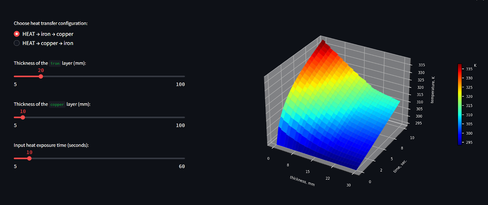
The temperature evolution across the plate was visualized using Python libraries:
- Matplotlib: Rendered 3D surface plots of temperature versus thickness and time.
- PyVista: Provided additional 3D visualizations for exploratory analysis.
The final output highlighted:
- Layered Effects: Differences in thermal conductivity and heat capacity between iron and copper significantly influenced heat transfer dynamics.
- Interface Dynamics: Temperature continuity and flux matching at the interface showcased the effects of material contrasts.
Key Observations
- Dynamic Adjustments: The interplay of material properties, boundary conditions, and time-dependent heat transfer resulted in non-linear temperature profiles.
- Material Dependency: Thermal properties, fetched dynamically using SplineCloud, played a pivotal role in determining the heat transfer behavior.
Conclusion
This study demonstrates a comprehensive, yet easy-to-use framework for analyzing non-steady heat conductivity in multi-layer systems. By combining Python's computational capabilities with SplineCloud's toolset, the model achieved high accuracy and adaptability.
The methodology can be extended to complex geometries and multi-material systems, offering valuable insights for industrial and scientific applications.
References
- Repository with material properties: https://splinecloud.com/repository/scorpaena/Metal_properties/
- Python Implementation: https://github.com/scorpaena/nonsteady_heat_conductivity
- Conduction Heat Transfer Solutions: https://digital.library.unt.edu/ark:/67531/metadc1110123/m2/1/high_res_d/6224569.pdf
- Numerical Methods in Heat, Mass, and Momentum Transfer: https://engineering.purdue.edu/~scalo/menu/teaching/me608/ME608_Notes_Murthy.pdf