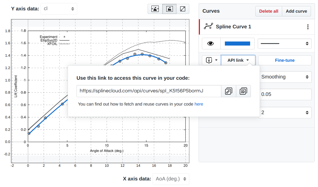
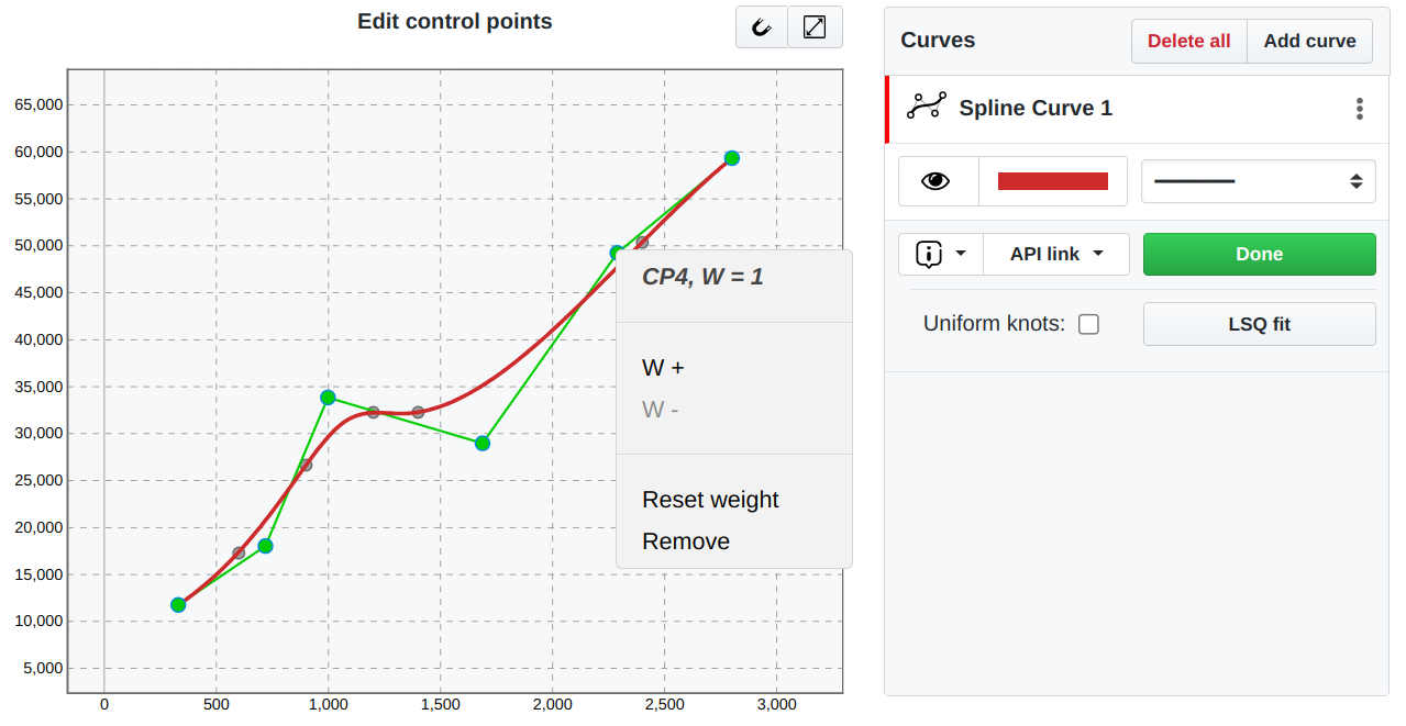
An Interactive Online Curve Fitting Tool
Improve Your Data Processing Workflow
with our free curve fitting software:
- build regression models interactively,
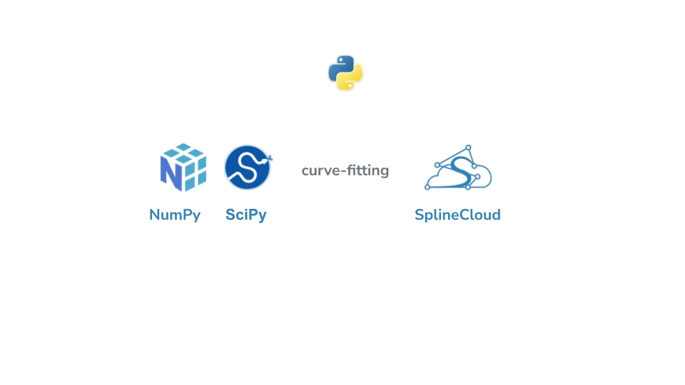
- reuse them in code,
- share models with your team.